Core CS Concept

Big-O Notation for CS Students

Asymptotic complexity analysis explained from the ground up. 8 common complexity classes from O(1) through O(2^n), Big-O vs Big-Theta vs Big-Omega distinctions, amortized analysis, and a cross-language benchmark table showing actual measured runtimes from n=10 through n=10,000 in Java, Python, C++, and JavaScript. Verified CS graduates from CMU, MIT, and Stanford, starting at $20 per task.

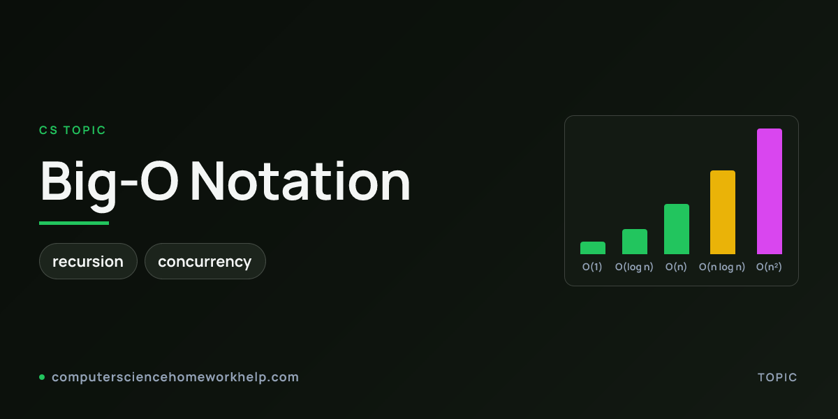
Big-O Notation concept visualization showing asymptotic time and space complexity analysis
4 Languages covered
10 FAQ answers
2 Related subjects
3 Code examples

What it means

A working definition of Big-O Notation

Big-O notation describes how an algorithm scales with input size, hiding constants and lower-order terms so the dominant growth rate stays visible at scale.

Same algorithm, different constants: Python is roughly 20x slower than C++, but the asymptotic class (O(n), O(n log n), O(n^2)) stays identical across Java, Python, C++, and JavaScript.

Primary example

Three complexity classes side by side

Three complexity classes side by side

          
          // O(1) constant - one operation regardless of input size
        
          
          public int firstElement(int[] arr) {
        
          
              return arr[0];
        
          
          }


          // O(n) linear - one pass through the input
        
          
          public int sum(int[] arr) {
        
          
              int total = 0;
        
          
              for (int x : arr) total += x;
        
          
              return total;
        
          
          }


          // O(n^2) quadratic - nested loop over input
        
          
          public boolean hasDuplicate(int[] arr) {
        
          
              for (int i = 0; i < arr.length; i++) {
        
          
                  for (int j = i + 1; j < arr.length; j++) {
        
          
                      if (arr[i] == arr[j]) return true;
        
          
                  }
        
          
              }
        
          
              return false;
        
          
          }
        

Three asymptotic bounds

Common big-o notation patterns

Big-O: upper bound

f(n) = O(g(n)) means f grows no faster than g, up to a constant factor and for large enough n. The standard claim in informal speech: "merge sort is O(n log n)" gives the worst-case ceiling.

Big-Theta: tight bound

f(n) = Theta(g(n)) bounds f both above and below by constant multiples of g. The complete claim for merge sort is Theta(n log n); CS161 graders deduct points for using O when Theta is provable.

Big-Omega: lower bound

f(n) = Omega(g(n)) means f grows no slower than g. Used to prove no algorithm can do better than a certain rate, like the comparison-sort Omega(n log n) decision-tree lower bound.

Cross-language

Same concept across languages

Python: 4 complexity classes
# O(1) constant - dict lookup
def get(d, key):
    return d.get(key)

# O(log n) logarithmic - binary search
def binary_search(arr, target):
    lo, hi = 0, len(arr) - 1
    while lo <= hi:
        mid = (lo + hi) // 2
        if arr[mid] == target: return mid
        if arr[mid] < target: lo = mid + 1
        else: hi = mid - 1
    return -1

# O(n log n) linearithmic - merge sort
def merge_sort(arr):
    if len(arr) <= 1: return arr
    mid = len(arr) // 2
    left = merge_sort(arr[:mid])
    right = merge_sort(arr[mid:])
    return merge(left, right)

# O(2^n) exponential - naive recursive Fibonacci
def fib(n):
    if n < 2: return n
    return fib(n - 1) + fib(n - 2)
C++: amortized O(1) push_back
// std::vector dynamic-array growth
// Most push_back calls are O(1); resize-and-copy is O(n).
// Amortized cost per push_back is O(1).

#include <vector>
std::vector<int> v;
for (int i = 0; i < 1000000; i++) {
    v.push_back(i);  // O(1) amortized
}

// Internal growth pattern (GCC libstdc++ default):
// capacity doubles when full: 1, 2, 4, 8, 16, ..., 524288, 1048576
// 20 resize events total for 1 million pushes
// Total work: 1+2+4+...+1048576 = 2097151 element copies
// Per push: 2097151 / 1000000 ~= 2.1 amortized copies

FAQ

Big-O Notation FAQ

What is the difference between Big-O and Big-Theta?
Big-O is an upper bound; Big-Theta is a tight bound. f(n) = O(g(n)) means f grows no faster than g, up to a constant factor and for large enough n. f(n) = Theta(g(n)) means f grows at exactly the same rate as g, both upper and lower bounded by constant multiples of g. Merge sort is O(n^2) (true but uninformative), O(n log n) (true and useful), and Theta(n log n) (the complete claim). CS161 graders deduct points for writing O when Theta is provable.
Why do constants disappear in Big-O notation?
Constants disappear because Big-O measures growth rate as input approaches infinity, not exact runtime. 100n and 2n are both O(n) because the ratio between them stays at 50:1 regardless of n. A linear-time algorithm with a 100x constant overhead still beats a quadratic-time algorithm once n is large enough; the crossover point depends on the constants, but for n above roughly 10000 the linear algorithm wins regardless. For small inputs, constants matter and Big-O can mislead: Java's Arrays.sort switches from quicksort to insertion sort for subarrays smaller than 47 because insertion sort's smaller constant beats quicksort's n log n at that scale.
How do I find the Big-O of a recursive algorithm?
Write the recurrence relation, then solve it with one of three methods. Substitution: guess the solution and prove it by induction. Recursion tree: draw the call tree, compute the work per level, and sum across levels. Master theorem: applies to T(n) = a T(n/b) + f(n) form; compare f(n) to n^log_b(a). Merge sort T(n) = 2 T(n/2) + n gives Theta(n log n) via master theorem case 2. Naive Fibonacci T(n) = T(n-1) + T(n-2) + 1 does not fit master theorem; substitute to get Theta(2^n) using the golden-ratio bound.
What is amortized analysis and when do I need it?
Amortized analysis bounds the average cost per operation over a sequence, when individual operations vary in cost. The canonical example is the dynamic array: push is O(n) when the array resizes but O(1) most of the time, and the amortized cost across n pushes is O(1). Three techniques formalize this: aggregate method (total cost divided by n operations), accounting method (assign credits per operation and prove the bank stays non-negative), potential method (define a potential function on data structure state). Other amortized examples: splay trees, Fibonacci heaps, Union-Find with path compression. Amortized bounds do not apply to real-time systems where every individual operation must finish in bounded time.
Is O(log n) faster than O(n) in practice?
Yes, dramatically so for large n. log_2(1,000,000) is 20, so a binary search on a million-element sorted array takes 20 comparisons; a linear search takes 1,000,000. The ratio grows: log_2(1 billion) is 30, log_2(1 trillion) is 40. For n below roughly 100, the difference is small enough that constants determine the winner; binary search has higher per-comparison overhead than linear scan because of pointer arithmetic and cache misses. Above n = 1000, log n complexity wins on any modern machine. Binary search requires a sorted array; if sorting takes O(n log n), the upfront cost beats repeated linear scans after a small number of queries.
What is the difference between worst-case and average-case complexity?
Worst-case complexity bounds runtime over the worst possible input of size n. Average-case complexity bounds expected runtime over a probability distribution of inputs. Quicksort with a random pivot has worst-case Theta(n^2) (adversarial input that always picks the smallest pivot) but expected Theta(n log n) over random permutations. Hash tables have worst-case Theta(n) lookup (every key hashes to the same bucket) but expected Theta(1) under universal hashing. Worst-case bounds are used for adversarial guarantees; average-case bounds are used for typical performance with caveats about the input distribution. CS161 problem sets ask for both when they differ.
How do I prove an algorithm is O(n) and not faster?
Prove a Big-Omega lower bound. For the input-reading lower bound: any algorithm that examines every element of an n-element input takes Omega(n) time, so an algorithm that must touch every element cannot be sub-linear. For comparison-based sorting: the decision-tree argument proves Omega(n log n) is a lower bound for any comparison sort, so merge sort and heap sort achieve the optimum. For the searching lower bound: any algorithm that searches an unsorted array for a specific value takes Omega(n) in the worst case, because the adversary can place the target last. Combining a matching Big-O upper bound with the Omega lower bound gives a Theta result, proving optimality.
What complexity is acceptable for a coding interview or autograder?
Compute the operations-per-second budget. C++ executes roughly 10^8 to 10^9 simple operations per second; Java around 10^8; Python around 10^6 to 10^7; JavaScript around 10^7 to 10^8. For a 1-second time limit and n = 100,000: O(n^2) needs 10^10 operations, exceeds budget in every language. O(n log n) needs 10^6 operations, comfortable in every language. O(n) needs 10^5 operations, comfortable. For n = 1,000,000: O(n^2) impossible, O(n log n) borderline in Python, O(n) comfortable. Match the algorithm complexity to the input size before writing code. Codeforces TLE (time limit exceeded) means the chosen complexity is wrong for the input; redesign to a lower complexity, do not micro-optimize the existing code.
How do I measure actual runtime to verify Big-O?
Run the algorithm on inputs of size n=10, 100, 1000, 10000 and plot runtime vs n. O(n) shows a straight line on linear axes. O(n log n) shows a nearly-linear curve. O(n^2) shows a parabola; doubling n quadruples runtime. O(2^n) shows exponential explosion; adding 1 to n doubles runtime. Use System.nanoTime in Java, time.perf_counter in Python, std::chrono::high_resolution_clock in C++, performance.now in JavaScript. Median of 10 runs eliminates outliers from garbage collection or thermal throttling. The measured curve should match the theoretical Big-O; if it does not, either the analysis is wrong or the constants are dominating at the chosen input sizes.
Can you help with master theorem and recurrence relations?
Yes. The master theorem solves T(n) = a T(n/b) + f(n) by comparing f(n) to n^log_b(a). Case 1: f(n) is polynomially smaller, T(n) = Theta(n^log_b(a)). Case 2: f(n) is equal up to log factors, T(n) = Theta(n^log_b(a) log^(k+1) n). Case 3: f(n) is polynomially larger and the regularity condition holds, T(n) = Theta(f(n)). Worked examples cover merge sort (case 2), binary search (case 2), Strassen multiplication (case 1), and Karatsuba multiplication (case 1). Non-master-theorem recurrences solved via substitution or recursion tree. Standard work on MIT 6.006 problem set 1, CS161 problem set 2, and CMU 15-451 problem sets.

Stuck on big-o notation?

Submit your assignment and get expert, pedagogical help within 12 hours. Every solution ships with line-by-line comments, complexity analysis, and unlimited revisions.

Get Big-O Notation Help