Per-structure cost tables
Arrays, linked lists, trees, heaps, hash maps, tries, graphs. Worst case, average, and space columns for every operation.
Reference
Time and space complexity for every common data structure and algorithm. Same operation shown across Java, Python, C++, and JavaScript so you can compare directly.
Overview
At a glance
Arrays, linked lists, trees, heaps, hash maps, tries, graphs. Worst case, average, and space columns for every operation.
Java, Python, C++, and JavaScript. Same operation across languages so you can pick the right container for your assignment.
Operations per second per language, what n fits in a 1-second timeout, and the 5 traps that lose Gradescope points.
Section 1 of 30
Each row uses Landau notation. O(f(n)) is the upper bound on growth, Θ(f(n)) is the tight bound, and Ω(f(n)) is the lower bound. Coursework almost always wants Big-O, so that is what every row reports. n is the input size, k is a secondary parameter (key length, alphabet size, bucket count), and V, E are the vertex and edge counts of a graph.
Amortized complexity assumes a long run of operations. A single Python list append can trigger an O(n) realloc when the backing array doubles. Across n appends, the total work is O(n), so the per-operation amortized cost is O(1). Always report worst case in coursework unless the prompt asks for amortized.
Asymptotics drop constants, but the autograder does not. A factor of 10 between a hash map and a tree map shows up as a wall-clock timeout on data-structures autograder problems with n above 10^6. The common compiler errors guide covers what causes the slowdown when the algorithm is theoretically the same.
Section 2 of 30
Arrays back nearly every other structure. Random access by index is O(1). Linear search by value is O(n). Append is amortized O(1) in dynamic arrays (Python list, Java ArrayList, C++ std::vector, JS Array) but O(n) when the backing buffer reallocates, which happens on a power-of-2 boundary in CPython and at a 1.5 growth factor in std::vector under libstdc++.
| Operation | Worst case | Average | Notes |
|---|---|---|---|
| Access by index | O(1) | O(1) | Pointer arithmetic on contiguous memory. |
| Search by value | O(n) | O(n) | Linear scan. Use a hash set if hot. |
| Insert at end | O(n) | O(1) | Realloc on grow. |
| Insert at front | O(n) | O(n) | Shifts every element. |
| Insert at index k | O(n) | O(n) | Shifts n-k elements. |
| Delete at end | O(1) | O(1) | Pop. |
| Delete at front | O(n) | O(n) | Shifts every element. |
A static array is fixed-size at allocation. A C array, a Java int[], a C++ std::array<T, N> are all static. Memory layout is contiguous, allocation is one block, and the size cannot change. Access and indexed write are strictly O(1) with no amortization.
A dynamic array wraps a static array plus a size counter and a capacity counter. When the size hits capacity, the implementation allocates a larger block (typically 2x or 1.5x the old capacity), memcpys the contents over, and frees the old block. The reallocation costs O(n), but amortized over n appends it costs O(1) per append. Python list, Java ArrayList, C++ std::vector, Go slice, Rust Vec are all dynamic arrays.
In C and C++, a 2D static array int grid[100][100] is contiguous in row-major order. Iterating row by row gets cache hits; iterating column by column gets cache misses on every access. A naive 1000x1000 matrix multiplication that iterates the second matrix column-major is 5x slower than the row-major version because of L1 cache thrashing.
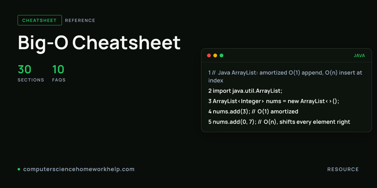
// Java ArrayList: amortized O(1) append, O(n) insert at index
import java.util.ArrayList;

ArrayList<Integer> nums = new ArrayList<>();
nums.add(3);          // O(1) amortized
nums.add(0, 7);       // O(n), shifts every element right
int first = nums.get(0); // O(1) random access
nums.remove(0);       // O(n), shifts every element left
boolean found = nums.contains(3); // O(n), linear scan# Python list: amortized O(1) append, O(n) insert at index
nums = []
nums.append(3) # O(1) amortized
nums.insert(0, 7) # O(n), shifts every element right
first = nums[0] # O(1) random access
del nums[0] # O(n), shifts every element left
found = 3 in nums # O(n), linear scan
# Gotcha: nums[1:] copies the tail (O(n)), not free slicing.// C++ std::vector: amortized O(1) push_back, O(n) insert at index
#include <vector>
#include <algorithm>
std::vector<int> nums;
nums.push_back(3); // O(1) amortized
nums.insert(nums.begin(), 7); // O(n)
int first = nums[0]; // O(1)
nums.erase(nums.begin()); // O(n)
auto it = std::find(nums.begin(), nums.end(), 3); // O(n)
bool found = (it != nums.end());// JavaScript Array: amortized O(1) push, O(n) unshift
const nums = [];
nums.push(3); // O(1) amortized
nums.unshift(7); // O(n), shifts every element right
const first = nums[0]; // O(1) random access
nums.shift(); // O(n), shifts every element left
const found = nums.includes(3); // O(n), linear scan
// V8 backs small arrays with packed C++ arrays; sparse arrays
// switch to a hash map (much slower).Section 3 of 30
Singly linked lists trade random access for cheap head insertion. Access at index k is O(k). Insert at head is O(1). Doubly linked lists also give O(1) tail insertion, at the cost of one extra pointer per node. The Java LinkedList class is doubly linked. C++ std::list is doubly linked; std::forward_list is singly linked and uses half the per-node memory.
| Operation | Singly | Doubly |
|---|---|---|
| Access at index k | O(k) | O(k) |
| Insert at head | O(1) | O(1) |
| Insert at tail (with tail pointer) | O(1) | O(1) |
| Insert before known node | O(n) (need predecessor) | O(1) |
| Delete known node | O(n) | O(1) |
| Search by value | O(n) | O(n) |
// Java LinkedList (doubly linked): O(1) head and tail ops
import java.util.LinkedList;

LinkedList<Integer> list = new LinkedList<>();
list.addFirst(1);  // O(1)
list.addLast(2);   // O(1) (tail pointer)
int head = list.getFirst(); // O(1)
int kth = list.get(3);      // O(k), walks from nearer end
list.removeFirst(); // O(1)# Python: no built-in linked list. collections.deque is a doubly
# linked list of fixed-size blocks. O(1) at both ends, O(n) in middle.
from collections import deque
q = deque()
q.appendleft(1) # O(1)
q.append(2) # O(1)
head = q[0] # O(1)
kth = q[3] # O(n) middle access
q.popleft() # O(1)// C++ std::list (doubly linked): O(1) splice, O(n) middle access
#include <list>
std::list<int> nums;
nums.push_front(1); // O(1)
nums.push_back(2); // O(1)
int head = nums.front(); // O(1)
auto it = nums.begin();
std::advance(it, 3); // O(k)
nums.erase(it); // O(1) given iterator// JavaScript: hand-rolled singly linked list
class Node {
constructor(v) { this.v = v; this.next = null; }
}
class LinkedList {
constructor() { this.head = null; }
prepend(v) { // O(1)
const n = new Node(v);
n.next = this.head;
this.head = n;
}
search(v) { // O(n)
let cur = this.head;
while (cur) {
if (cur.v === v) return cur;
cur = cur.next;
}
return null;
}
}Section 4 of 30
Stacks expose push, pop, peek. All 3 run in O(1) on a dynamic array backing, amortized for push when the buffer grows. Queues expose enqueue, dequeue, peek. Naive array-backed queues hit O(n) on dequeue because every element shifts. Use a deque or a ring buffer.
The Java ArrayDeque is the recommended stack and queue in modern code. The older java.util.Stack class extends Vector and inherits synchronized methods, which slows hot paths. Python users reach for collections.deque; both ends are O(1).
A ring buffer (circular buffer) is a fixed-size array with two indices (head and tail) that wrap modulo capacity. Enqueue, dequeue, and access by offset are all O(1). Used in producer-consumer queues, audio buffers, and network packet queues. The Linux kernel uses ring buffers for the perf event subsystem and the io_uring async I/O interface.
A monotonic stack maintains its elements in sorted order by popping any element that would break the invariant. Used in the classic problems "next greater element" and "largest rectangle in histogram" to get an O(n) solution where naive nested loops give O(n^2). A monotonic deque generalizes the pattern to sliding-window problems like "max of every k-sized window" in O(n) total.
// Java ArrayDeque as stack and queue: O(1) on both ends
import java.util.ArrayDeque;

ArrayDeque<Integer> stack = new ArrayDeque<>();
stack.push(1); stack.push(2);     // O(1) amortized
int top = stack.pop();            // O(1)

ArrayDeque<Integer> queue = new ArrayDeque<>();
queue.offer(1); queue.offer(2);   // O(1)
int head = queue.poll(); // O(1)# Python deque: O(1) at both ends
from collections import deque
stack = deque()
stack.append(1) # O(1) push
top = stack.pop() # O(1)
queue = deque()
queue.append(1) # O(1) enqueue
head = queue.popleft() # O(1) dequeue
# Anti-pattern: queue = list(); queue.pop(0) is O(n).// C++ std::stack and std::queue are adapters over std::deque
#include <stack>
#include <queue>
std::stack<int> s;
s.push(1); s.push(2); // O(1) amortized
int top = s.top(); // O(1)
s.pop(); // O(1)
std::queue<int> q;
q.push(1); q.push(2); // O(1)
int head = q.front(); // O(1)
q.pop(); // O(1)Section 5 of 30
An unbalanced BST degrades to O(n) on sorted insertions because every node becomes a right child. Self-balancing trees (AVL, red-black, B-tree) restore the O(log n) guarantee per operation. The Java TreeMap and C++ std::map are red-black trees. Python has no built-in balanced tree; use sortedcontainers.SortedDict from the third-party sortedcontainers package or fall back to a heap when ordering is all you need.
| Tree type | Search | Insert | Delete | Notes |
|---|---|---|---|---|
| Unbalanced BST | O(n) | O(n) | O(n) | Pathological on sorted input. |
| AVL | O(log n) | O(log n) | O(log n) | Stricter balance, faster search. |
| Red-black | O(log n) | O(log n) | O(log n) | Looser balance, faster insert. |
| B-tree (order m) | O(log_m n) | O(log_m n) | O(log_m n) | Optimized for disk pages. |
// Java TreeMap is a red-black tree: O(log n) ordered map
import java.util.TreeMap;

TreeMap<Integer, String> map = new TreeMap<>();
map.put(5, "five");   // O(log n)
map.put(2, "two");    // O(log n)
String v = map.get(5); // O(log n)
Integer first = map.firstKey(); // O(log n)
Integer ceil = map.ceilingKey(3); // O(log n), smallest >= 3// C++ std::map is a red-black tree: O(log n)
#include <map>
std::map<int, std::string> m;
m[5] = "five"; // O(log n)
m[2] = "two"; // O(log n)
auto it = m.find(5); // O(log n)
auto lb = m.lower_bound(3); // O(log n), first key >= 3
// Iterating in order is O(n).# Python sorted dict via sortedcontainers (third-party)
from sortedcontainers import SortedDict
sd = SortedDict()
sd[5] = "five" # O(log n)
sd[2] = "two" # O(log n)
v = sd[5] # O(log n)
first = sd.peekitem(0) # O(log n)
# Built-in dict is hash-based: O(1) avg, but unordered by key.Section 6 of 30
A binary heap is a complete binary tree backed by an array. Peek is O(1). Insert and extract are O(log n) due to sift-up and sift-down. Build-heap from an unsorted array is O(n), not O(n log n) (Floyd build). Use a heap for top-K problems, Dijkstra, A*, and median-maintenance via twin heaps.
For a node at index i in the backing array (1-indexed): the parent is at i/2, the left child is at 2i, and the right child is at 2i+1. With 0-indexing: parent is (i-1)/2, children are 2i+1 and 2i+2. No pointers stored, no auxiliary tree structure; the array indices encode the parent-child relationship for free.
| Heap type | Find-min | Insert | Decrease-key | Extract-min |
|---|---|---|---|---|
| Binary heap | O(1) | O(log n) | O(log n) | O(log n) |
| Binomial heap | O(log n) | O(log n) amortized O(1) | O(log n) | O(log n) |
| Fibonacci heap | O(1) | O(1) amortized | O(1) amortized | O(log n) amortized |
| Pairing heap | O(1) | O(1) | O(log n) (open) | O(log n) amortized |
Fibonacci heaps give the asymptotically best Dijkstra implementation but the constant factor is so large that binary heaps are faster on graphs with up to ~10^6 vertices. Use a binary heap by default; reach for Fibonacci only when the algorithm explicitly needs O(1) decrease-key for a theoretical result.
// Java PriorityQueue (min-heap by default)
import java.util.PriorityQueue;
import java.util.Collections;

PriorityQueue<Integer> minHeap = new PriorityQueue<>();
minHeap.offer(5);          // O(log n) sift-up
minHeap.offer(2);          // O(log n)
int min = minHeap.peek();   // O(1)
minHeap.poll();             // O(log n) sift-down

// Max-heap via reverse comparator
PriorityQueue<Integer> maxHeap = new PriorityQueue<>(Collections.reverseOrder());# Python heapq is a min-heap. For max-heap, negate keys.
import heapq
nums = [5, 2, 8, 1]
heapq.heapify(nums) # O(n) Floyd build
heapq.heappush(nums, 3) # O(log n)
smallest = nums[0] # O(1) peek
heapq.heappop(nums) # O(log n)
# Top 3 smallest
top3 = heapq.nsmallest(3, [5, 2, 8, 1, 9]) # O(n log k)// C++ std::priority_queue is a max-heap by default
#include <queue>
#include <vector>
std::priority_queue<int> maxHeap;
maxHeap.push(5); // O(log n)
maxHeap.push(2); // O(log n)
int top = maxHeap.top(); // O(1)
maxHeap.pop(); // O(log n)
// Min-heap with greater<int>
#include <functional>
std::priority_queue<int, std::vector<int>, std::greater<int>> minHeap;Section 7 of 30
Hash tables give O(1) average for insert, search, and delete. Worst case is O(n) when every key collides into one bucket. Coursework almost always assumes the average case. Real benchmarks reveal the worst case under adversarial input, which is why CPython randomizes hash seeds for strings (PEP 456) and Java HashMap converts a bucket to a red-black tree after 8 collisions (since Java 8).
| Map | Backed by | Insert avg | Insert worst | Ordered iteration |
|---|---|---|---|---|
| Java HashMap | array + linked list, treeifies at 8 | O(1) | O(log n) | No |
| Java TreeMap | red-black tree | O(log n) | O(log n) | Yes |
| Python dict | open addressing, probing | O(1) | O(n) | Insertion order (3.7+) |
| C++ unordered_map | chaining | O(1) | O(n) | No |
| C++ map | red-black tree | O(log n) | O(log n) | Yes |
The load factor is the ratio of stored items to buckets. Java HashMap resizes when load factor exceeds 0.75. Python dict resizes at 2/3. Resize costs O(n) (rehash every existing entry into the new larger bucket array) but happens only O(log n) times across n inserts, so amortized insert stays O(1).
Two collision-resolution strategies. Separate chaining stores collided entries in a linked list (or, in Java 8+, a tree) per bucket. Open addressing probes alternate buckets (linear probing, quadratic probing, double hashing) until it finds an empty one. Python dict uses open addressing with perturbation probing for better cache locality. Java HashMap uses separate chaining for simpler resize logic. Open addressing wins on cache; chaining wins on resize and high load factors.
// Java HashMap: O(1) average, O(log n) worst since Java 8
import java.util.HashMap;

HashMap<String, Integer> grades = new HashMap<>();
grades.put("Ada", 95);   // O(1) avg
grades.put("Bob", 82);   // O(1) avg
int n = grades.get("Ada"); // O(1) avg
boolean has = grades.containsKey("Cy"); // O(1) avg# Python dict: O(1) average. PEP 456 randomizes seed.
grades = {}
grades["Ada"] = 95 # O(1) avg
grades["Bob"] = 82 # O(1) avg
n = grades["Ada"] # O(1) avg
has = "Cy" in grades # O(1) avg
# Adversarial worst case: O(n^2) for n insertions if hashes collide.// C++ unordered_map: chaining, O(1) average
#include <unordered_map>
#include <string>
std::unordered_map<std::string, int> grades;
grades["Ada"] = 95; // O(1) avg
grades["Bob"] = 82; // O(1) avg
int n = grades["Ada"]; // O(1) avg
bool has = grades.count("Cy") > 0; // O(1) avg// JavaScript Map: O(1) average insert and get
const grades = new Map();
grades.set("Ada", 95); // O(1) avg
grades.set("Bob", 82); // O(1) avg
const n = grades.get("Ada"); // O(1) avg
const has = grades.has("Cy"); // O(1) avg
// Plain object {} also works as a map, but Map preserves
// insertion order across all key types, not just strings.Section 8 of 30
The default sort in every major language is comparison-based and runs in O(n log n) average time. The constant factors and worst-case behavior differ.
| Language | Algorithm | Worst case | Stable | In-place |
|---|---|---|---|---|
Python sorted, list.sort | Timsort | O(n log n) | Yes | Yes (sort), No (sorted) |
Java Arrays.sort (objects) | Timsort | O(n log n) | Yes | Yes |
Java Arrays.sort (primitives) | Dual-pivot quicksort | O(n log n) | No | Yes |
C++ std::sort | Introsort (quicksort + heapsort) | O(n log n) | No | Yes |
C++ std::stable_sort | Mergesort variant | O(n log n) | Yes | No (needs O(n) aux) |
| JS Array.prototype.sort (V8) | Timsort (since 2019) | O(n log n) | Yes | Yes |
Mergesort allocates a buffer the size of the input so the merge step can read two sorted halves into one output. Quicksort sorts in place but recurses O(log n) deep; introsort detects pathological splits and switches to heapsort to guarantee O(n log n) worst case.
# Python Timsort: stable, O(n log n), O(n) aux
nums = [3, 1, 4, 1, 5, 9, 2, 6]
nums.sort()                      # in place, returns None
print(nums)                      # [1, 1, 2, 3, 4, 5, 6, 9]
out = sorted(nums, reverse=True) # returns new list
print(out)                       # [9, 6, 5, 4, 3, 2, 1, 1]

# Sort by key (stable preserves original order on ties)
people = [("Ada", 30), ("Bob", 25), ("Ada", 22)]
people.sort(key=lambda p: p[0])
print(people) # Ada-30 before Ada-22 (stable)// Java Arrays.sort: dual-pivot quicksort for primitives,
// Timsort for object arrays.
import java.util.Arrays;
import java.util.Comparator;
int[] nums = {3, 1, 4, 1, 5, 9, 2, 6};
Arrays.sort(nums); // dual-pivot quicksort
System.out.println(Arrays.toString(nums));
Integer[] boxed = {3, 1, 4, 1, 5, 9, 2, 6};
Arrays.sort(boxed, Comparator.reverseOrder()); // Timsort, stable// C++ std::sort: introsort, O(n log n) worst case
#include <algorithm>
#include <vector>
std::vector<int> nums = {3, 1, 4, 1, 5, 9, 2, 6};
std::sort(nums.begin(), nums.end()); // ascending
std::sort(nums.begin(), nums.end(), std::greater<int>()); // descending
// std::stable_sort preserves equal-key order, uses O(n) aux memory
std::stable_sort(nums.begin(), nums.end());// JavaScript Array.prototype.sort: Timsort in V8 since 2019
const nums = [3, 1, 4, 1, 5, 9, 2, 6];
nums.sort((a, b) => a - b);
console.log(nums); // [1, 1, 2, 3, 4, 5, 6, 9]
// Gotcha: nums.sort() with no comparator coerces to strings:
// [10, 2, 1].sort() returns [1, 10, 2], not [1, 2, 10].Section 9 of 30
Linear search is O(n) and needs no precondition. Binary search is O(log n) on a sorted random-access container. Interpolation search is O(log log n) on uniformly distributed sorted data, degrading to O(n) on skewed distributions. The wall-clock crossover: linear beats binary for n below roughly 100 because the constant factor in binary search (branch mispredictions on the midpoint compare) outweighs the algorithmic win.
# Python bisect: O(log n) binary search on sorted list
import bisect

nums = [1, 3, 5, 7, 9, 11]
idx = bisect.bisect_left(nums, 5)   # 2 (insertion point)
exists = idx < len(nums) and nums[idx] == 5
print(exists, idx)  # True 2

# Roll your own
def binary_search(arr, target):
    lo, hi = 0, len(arr) - 1
    while lo <= hi:
        mid = (lo + hi) // 2
        if arr[mid] == target: return mid
        if arr[mid] < target: lo = mid + 1
        else: hi = mid - 1
return -1// Java Arrays.binarySearch: O(log n)
import java.util.Arrays;
int[] nums = {1, 3, 5, 7, 9, 11};
int idx = Arrays.binarySearch(nums, 5);
System.out.println(idx); // 2
// Returns -(insertion_point + 1) if not found
int missing = Arrays.binarySearch(nums, 4); // -3 means insert at index 2// C++ std::binary_search and std::lower_bound: O(log n)
#include <algorithm>
#include <vector>
std::vector<int> nums = {1, 3, 5, 7, 9, 11};
bool found = std::binary_search(nums.begin(), nums.end(), 5);
auto it = std::lower_bound(nums.begin(), nums.end(), 5);
int idx = it - nums.begin(); // 2Section 10 of 30
Graph algorithm complexity always reads O(V + E) or worse. The vertex count V and edge count E dominate. BFS and DFS are O(V + E). Dijkstra with a binary heap is O((V + E) log V). Bellman-Ford is O(V * E) but handles negative edge weights. Floyd-Warshall is O(V^3) and gives all-pairs shortest paths. A* matches Dijkstra in worst case but visits fewer nodes with an admissible heuristic.
| Algorithm | Time | Space | Handles negative edges | Detects negative cycles |
|---|---|---|---|---|
| BFS (unweighted) | O(V + E) | O(V) | N/A | N/A |
| Dijkstra (binary heap) | O((V + E) log V) | O(V) | No | No |
| Dijkstra (Fibonacci heap) | O(V log V + E) | O(V) | No | No |
| Bellman-Ford | O(V * E) | O(V) | Yes | Yes |
| Floyd-Warshall (all-pairs) | O(V^3) | O(V^2) | Yes | Yes |
# BFS on an adjacency list: O(V + E)
from collections import deque

def bfs(graph, start):
    visited = {start}
    q = deque([start])
    order = []
    while q:
        u = q.popleft()
        order.append(u)
        for v in graph[u]:
            if v not in visited:
                visited.add(v)
                q.append(v)
    return order

graph = {'A': ['B', 'C'], 'B': ['D'], 'C': ['D'], 'D': []}
print(bfs(graph, 'A')) # ['A', 'B', 'C', 'D']# Dijkstra with heapq: O((V + E) log V)
import heapq
def dijkstra(graph, source):
dist = {v: float('inf') for v in graph}
dist[source] = 0
pq = [(0, source)]
while pq:
d, u = heapq.heappop(pq)
if d > dist[u]:
continue
for v, w in graph[u]:
nd = d + w
if nd < dist[v]:
dist[v] = nd
heapq.heappush(pq, (nd, v))
return dist
g = {'A': [('B', 4), ('C', 1)],
'B': [('D', 1)],
'C': [('B', 2), ('D', 5)],
'D': []}
print(dijkstra(g, 'A')) # {'A': 0, 'B': 3, 'C': 1, 'D': 4}// Java BFS with adjacency list: O(V + E)
import java.util.*;
public List<Integer> bfs(List<List<Integer>> graph, int start) {
List<Integer> order = new ArrayList<>();
boolean[] seen = new boolean[graph.size()];
Deque<Integer> q = new ArrayDeque<>();
q.offer(start);
seen[start] = true;
while (!q.isEmpty()) {
int u = q.poll();
order.add(u);
for (int v : graph.get(u)) {
if (!seen[v]) {
seen[v] = true;
q.offer(v);
}
}
}
return order;
}// C++ Dijkstra with priority_queue: O((V + E) log V)
#include <queue>
#include <vector>
#include <limits>
std::vector<int> dijkstra(
const std::vector<std::vector<std::pair<int,int>>>& graph, int src) {
int n = graph.size();
std::vector<int> dist(n, std::numeric_limits<int>::max());
dist[src] = 0;
std::priority_queue<std::pair<int,int>,
std::vector<std::pair<int,int>>,
std::greater<>> pq;
pq.push({0, src});
while (!pq.empty()) {
auto [d, u] = pq.top(); pq.pop();
if (d > dist[u]) continue;
for (auto [v, w] : graph[u]) {
if (d + w < dist[v]) {
dist[v] = d + w;
pq.push({dist[v], v});
}
}
}
return dist;
}Section 11 of 30
Dynamic programming converts an exponential recursion into a polynomial table walk. The total work is (number of unique subproblems) * (cost per subproblem). Classic Fibonacci is O(n) time and O(1) space with rolling variables. Knapsack is O(n*W) where W is the capacity. Longest common subsequence is O(m*n). Edit distance is O(m*n) time and O(min(m,n)) space with row-rolling.
# Fibonacci: 3 implementations on a Big-O spectrum
def fib_naive(n):                # O(2^n) time, O(n) stack
    if n < 2: return n
    return fib_naive(n - 1) + fib_naive(n - 2)

def fib_memo(n, cache=None):     # O(n) time, O(n) space
    if cache is None: cache = {}
    if n in cache: return cache[n]
    if n < 2: return n
    cache[n] = fib_memo(n - 1, cache) + fib_memo(n - 2, cache)
    return cache[n]

def fib_iter(n):                 # O(n) time, O(1) space
    a, b = 0, 1
    for _ in range(n): a, b = b, a + b
return a# 0/1 knapsack: O(n*W) time, O(W) space with row-rolling
def knapsack(weights, values, capacity):
dp = [0] * (capacity + 1)
for i in range(len(weights)):
for w in range(capacity, weights[i] - 1, -1):
dp[w] = max(dp[w], dp[w - weights[i]] + values[i])
return dp[capacity]
print(knapsack([2, 3, 4, 5], [3, 4, 5, 6], 5)) # 7// Edit distance (Levenshtein): O(m*n) time, O(min(m,n)) space
public int editDistance(String s, String t) {
int m = s.length(), n = t.length();
int[] prev = new int[n + 1];
int[] curr = new int[n + 1];
for (int j = 0; j <= n; j++) prev[j] = j;
for (int i = 1; i <= m; i++) {
curr[0] = i;
for (int j = 1; j <= n; j++) {
int cost = s.charAt(i-1) == t.charAt(j-1) ? 0 : 1;
curr[j] = Math.min(
Math.min(curr[j-1] + 1, prev[j] + 1),
prev[j-1] + cost);
}
int[] tmp = prev; prev = curr; curr = tmp;
}
return prev[n];
}Section 12 of 30
Recursion costs O(depth) stack frames. Quicksort recurses O(log n) deep on balanced splits, O(n) deep on pathological splits. Mergesort recurses O(log n) deep but allocates O(n) extra buffer. Tail-recursive functions in Python and Java do not get optimized; the JVM and CPython preserve the stack. Scala, Scheme, and OCaml do tail-call optimization. C++ does it inconsistently across compilers and optimization levels.
A recursive function that recurses O(n) deep on a 2 MB default Linux thread stack typically blows the stack at n above 10^5. Iterative reformulation with an explicit stack avoids the limit.
Each stack frame holds saved registers, the return address, the locals, and any spilled arguments. A typical x86-64 frame is 64 to 256 bytes. A 2 MB stack with 128-byte frames bottoms out at 16,000 frames; with 64-byte frames, 32,000 frames. Compiler optimization (especially -O2) shrinks frame size by keeping more locals in registers. This is why a recursive Fibonacci compiled with -O0 blows the stack at n = 8,000 but the same code with -O2 reaches n = 20,000.
# Python recursion limit is 1000 by default
import sys
print(sys.getrecursionlimit())  # 1000
sys.setrecursionlimit(10**6)    # rare; usually rewrite iteratively

# Iterative DFS: O(V + E) time, O(V) explicit stack
def dfs_iter(graph, start):
    stack = [start]
    seen = {start}
    order = []
    while stack:
        u = stack.pop()
        order.append(u)
        for v in graph[u]:
            if v not in seen:
                seen.add(v)
                stack.append(v)
return order// Java has no TCO. Iterative tree traversal beats deep recursion.
import java.util.ArrayDeque;
import java.util.Deque;
void iterativeInorder(TreeNode root) {
Deque<TreeNode> stack = new ArrayDeque<>();
TreeNode cur = root;
while (cur != null || !stack.isEmpty()) {
while (cur != null) {
stack.push(cur);
cur = cur.left;
}
cur = stack.pop();
System.out.println(cur.val);
cur = cur.right;
}
}Section 13 of 30
Two algorithmic patterns convert nested-loop O(n^2) solutions into single-pass O(n) solutions on sorted or windowed input.
Initialize two pointers at the start and end (or at the same start). Move them based on a condition until they meet. Solves problems like "pair with sum k", "container with most water", "remove duplicates in sorted array" in O(n) where the brute force is O(n^2). Requires sorted input or a structure that supports the comparison.
Maintain a window [left, right] that expands or contracts based on the condition. Solves problems like "longest substring without repeating", "minimum window substring", "max sum of k consecutive". The window invariant is checked in O(1) per pointer move, totaling O(n) for the whole pass.
# Two-pointer: pair with sum k in sorted array, O(n)
def two_sum_sorted(nums, target):
    lo, hi = 0, len(nums) - 1
    while lo < hi:
        s = nums[lo] + nums[hi]
        if s == target: return (lo, hi)
        if s < target: lo += 1
        else: hi -= 1
    return None

# Sliding window: longest substring without repeating chars, O(n)
def longest_unique_substring(s):
    seen = {}
    left = best = 0
    for right, ch in enumerate(s):
        if ch in seen and seen[ch] >= left:
            left = seen[ch] + 1
        seen[ch] = right
        best = max(best, right - left + 1)
    return best

print(longest_unique_substring("abcabcbb"))  # 3 ("abc")
Section 14 of 30
Amortized cost is the average per-operation cost across a worst-case sequence. Aggregate method: sum the total cost, divide by the operation count. Banker method: every cheap op deposits credits, expensive ops withdraw them. Accounting method: assign each op a fictional charge equal to its amortized cost, surplus charges pay for future expensive ops.
# Union-Find with path compression and union by rank
# Amortized O(alpha(n)) per op (effectively constant)
class UnionFind:
    def __init__(self, n):
        self.parent = list(range(n))
        self.rank = [0] * n
    def find(self, x):
        root = x
        while self.parent[root] != root:
            root = self.parent[root]
        # path compression
        while self.parent[x] != root:
            self.parent[x], x = root, self.parent[x]
        return root
    def union(self, x, y):
        rx, ry = self.find(x), self.find(y)
        if rx == ry: return False
        if self.rank[rx] < self.rank[ry]: rx, ry = ry, rx
        self.parent[ry] = rx
        if self.rank[rx] == self.rank[ry]: self.rank[rx] += 1
        return True
Section 15 of 30
Many recursive algorithms have the recurrence T(n) = a T(n/b) + f(n), where a is the number of recursive calls, b is the input division factor, and f(n) is the work outside the recursive calls. The master theorem gives a closed-form answer in three cases.
| Algorithm | Recurrence | Solution | Case |
|---|---|---|---|
| Mergesort | T(n) = 2 T(n/2) + Θ(n) | Θ(n log n) | 2 |
| Binary search | T(n) = T(n/2) + Θ(1) | Θ(log n) | 2 |
| Strassen matrix mult | T(n) = 7 T(n/2) + Θ(n^2) | Θ(n^(log_2 7)) ≈ Θ(n^2.807) | 1 |
| Karatsuba multiplication | T(n) = 3 T(n/2) + Θ(n) | Θ(n^(log_2 3)) ≈ Θ(n^1.585) | 1 |
| Naive matrix mult divide-conquer | T(n) = 8 T(n/2) + Θ(n^2) | Θ(n^3) | 1 |
| Quickselect avg case | T(n) = T(n/2) + Θ(n) | Θ(n) | 3 |
The master theorem does not cover every recurrence. For T(n) = T(n-1) + n (selection sort recursion), use induction or the recursion tree method. Akra-Bazzi extends the master theorem to unequal subproblem sizes.
Section 16 of 30
An algorithm is in P if it runs in polynomial time (O(n^k) for some constant k). NP is the class of problems whose solutions can be verified in polynomial time. NP-complete problems are the hardest in NP: every NP problem reduces to them in polynomial time. If any NP-complete problem has a polynomial-time algorithm, P = NP and every NP problem becomes tractable. No one has found one in 50 years, and most researchers believe none exists.
If an assignment hands you what looks like an NP-complete problem, the expected solution is usually an approximation algorithm (within a constant factor of optimal), a branch-and-bound exact solver that runs fast on practical inputs, or a heuristic like simulated annealing or genetic algorithms. Brute force is fine for n below 20; exponential blowup kicks in around n = 30 on commodity hardware.
Section 17 of 30
Five mistakes show up in over 60% of failed Gradescope autograder submissions on intro data-structures courses, based on the patterns the CSHH tutoring team sees in the debug queue.
list.pop(0) in Python is O(n). list.contains(x) in Java is O(n). Either inside a for-loop turns an apparent O(n) algorithm into O(n^2).
Java String is immutable; s += "x" in a loop is O(n^2). Use StringBuilder. Python is the same for most CPython versions, despite occasional CPython optimizations that compress chained concatenations. "".join(parts) is the safe pattern.
Building a set inside a loop costs O(m) per iteration where m is the set size. Build once outside the loop.
Recursive Fibonacci is O(2^n), not O(n). Memoize or iterate.
Recursive mergesort uses O(n log n) total stack and buffer in the wrong implementation. In-place quicksort uses O(log n) stack. Autograders with a stack-depth limit reject the wrong choice.
# Anti-pattern: O(n^2) list.pop(0)
def remove_evens_bad(nums):
    i = 0
    while i < len(nums):
        if nums[i] % 2 == 0:
            nums.pop(i)        # O(n)
        else:
            i += 1
    # Total: O(n^2)

# Fixed: list comprehension is O(n)
def remove_evens_good(nums):
return [x for x in nums if x % 2 != 0]// Anti-pattern: O(n^2) string concat in loop
String build_bad(String[] parts) {
String out = "";
for (String p : parts) {
out += p; // each += creates a new String
}
return out;
}
// Fixed: StringBuilder is O(n)
String build_good(String[] parts) {
StringBuilder sb = new StringBuilder();
for (String p : parts) sb.append(p);
return sb.toString();
}Section 18 of 30
A trie (prefix tree) stores strings by character at each level. Insert is O(L) where L is the string length, independent of the trie size. Search is O(L). Prefix queries are O(L + k) where k is the number of results. Space cost is O(sum of all string lengths) in the worst case, far less when strings share prefixes.
A hash set answers exact-membership queries in O(1) but cannot do prefix queries without scanning all n keys (O(n * L) work). A trie answers both exact membership and prefix in O(L). For autocomplete with a million-word dictionary and queries returning 10 results, the trie wins by 5 orders of magnitude on the prefix-query path.
# Trie implementation: O(L) insert and search
class TrieNode:
    __slots__ = ('children', 'is_word')
    def __init__(self):
        self.children = {}
        self.is_word = False

class Trie:
    def __init__(self):
        self.root = TrieNode()
    def insert(self, word):       # O(L)
        node = self.root
        for ch in word:
            if ch not in node.children:
                node.children[ch] = TrieNode()
            node = node.children[ch]
        node.is_word = True
    def search(self, word):       # O(L)
        node = self.root
        for ch in word:
            if ch not in node.children: return False
            node = node.children[ch]
        return node.is_word
    def starts_with(self, prefix):  # O(L)
        node = self.root
        for ch in prefix:
            if ch not in node.children: return False
            node = node.children[ch]
return True// Java trie with array children for ASCII lowercase: faster than HashMap
class Trie {
static class Node {
Node[] children = new Node[26];
boolean isWord;
}
Node root = new Node();
void insert(String word) { // O(L)
Node cur = root;
for (char c : word.toCharArray()) {
int idx = c - 'a';
if (cur.children[idx] == null) cur.children[idx] = new Node();
cur = cur.children[idx];
}
cur.isWord = true;
}
boolean search(String word) { // O(L)
Node n = walk(word);
return n != null && n.isWord;
}
boolean startsWith(String prefix) { // O(L)
return walk(prefix) != null;
}
private Node walk(String s) {
Node cur = root;
for (char c : s.toCharArray()) {
int idx = c - 'a';
if (cur.children[idx] == null) return null;
cur = cur.children[idx];
}
return cur;
}
}Section 19 of 30
Three structures dominate the range-query category in competitive programming and database internals.
| Structure | Build | Point update | Range query | Space |
|---|---|---|---|---|
| Naive prefix sum | O(n) | O(n) (rebuild) | O(1) | O(n) |
| Fenwick tree (BIT) | O(n log n) | O(log n) | O(log n) | O(n) |
| Segment tree | O(n) | O(log n) | O(log n) | O(4n) |
| Segment tree + lazy | O(n) | O(log n) | O(log n) range update | O(4n) |
| Union-Find | O(n) | O(α(n)) | O(α(n)) find | O(n) |
The Fenwick tree is the smallest implementation for prefix-sum-with-updates. The segment tree handles arbitrary associative range queries (min, max, gcd, range XOR). Lazy propagation extends segment trees to support range updates, useful for difference-array problems and 2D rectangle queries.
# Fenwick tree (Binary Indexed Tree): O(log n) update and query
class Fenwick:
    def __init__(self, n):
        self.n = n
        self.tree = [0] * (n + 1)
    def update(self, i, delta):        # O(log n)
        i += 1
        while i <= self.n:
            self.tree[i] += delta
            i += i & -i
    def query(self, i):                # O(log n), prefix sum [0..i]
        i += 1
        s = 0
        while i > 0:
            s += self.tree[i]
            i -= i & -i
        return s
    def range_sum(self, l, r):         # O(log n)
return self.query(r) - (self.query(l - 1) if l > 0 else 0)// Segment tree with point update and range sum query: O(log n)
#include <vector>
class SegTree {
int n;
std::vector<long long> tree;
public:
SegTree(int n) : n(n), tree(4 * n, 0) {}
void update(int idx, long long val) { update(1, 0, n - 1, idx, val); }
long long query(int l, int r) { return query(1, 0, n - 1, l, r); }
private:
void update(int node, int lo, int hi, int idx, long long val) {
if (lo == hi) { tree[node] = val; return; }
int mid = (lo + hi) / 2;
if (idx <= mid) update(2*node, lo, mid, idx, val);
else update(2*node+1, mid+1, hi, idx, val);
tree[node] = tree[2*node] + tree[2*node+1];
}
long long query(int node, int lo, int hi, int l, int r) {
if (r < lo || hi < l) return 0;
if (l <= lo && hi <= r) return tree[node];
int mid = (lo + hi) / 2;
return query(2*node, lo, mid, l, r) + query(2*node+1, mid+1, hi, l, r);
}
};Section 20 of 30
Naive substring search is O(n*m) where n is the text length and m is the pattern length. Three specialized algorithms reduce this.
| Algorithm | Preprocess | Search | Best for |
|---|---|---|---|
| Naive | O(1) | O(n*m) | Very short patterns |
| KMP | O(m) | O(n + m) | Single pattern, long text |
| Rabin-Karp | O(m) | O(n + m) average, O(n*m) worst | Multiple patterns, plagiarism detection |
| Boyer-Moore | O(m + σ) | O(n/m) best, O(n*m) worst | Long patterns, sublinear average |
| Suffix array (construction) | O(n log n) | O(m log n) per query | Many queries against fixed text |
| Suffix automaton | O(n) | O(m) per query | Same, smaller constant |
MOSS (the plagiarism detector used at over 200 universities) is essentially a tuned Rabin-Karp over code tokens, using rolling hashes to detect duplicated k-grams across millions of submissions in O(N) total work.
# KMP substring search: O(n + m) time, O(m) preprocessing
def kmp_search(text, pattern):
    if not pattern: return 0
    # Build failure function
    fail = [0] * len(pattern)
    k = 0
    for i in range(1, len(pattern)):
        while k > 0 and pattern[k] != pattern[i]:
            k = fail[k - 1]
        if pattern[k] == pattern[i]:
            k += 1
        fail[i] = k
    # Search
    j = 0
    for i in range(len(text)):
        while j > 0 and pattern[j] != text[i]:
            j = fail[j - 1]
        if pattern[j] == text[i]:
            j += 1
        if j == len(pattern):
            return i - j + 1
    return -1

print(kmp_search("ABCABCABABC", "ABCAB"))  # 0
Section 21 of 30
Every bitwise operation is O(1) on a word-sized integer. x & y, x | y, x ^ y, ~x, x << k, x >> k all run in a single CPU cycle on 32 or 64 bit integers. On arbitrary-precision integers (Python int), the cost scales with the bit length, so the operation is O(b) where b is the bit count.
Branchless code replaces conditional jumps with bitwise expressions. The asymptotic cost stays the same but the constant drops by 2 to 5x on hot paths because branch mispredictions disappear. This is why competitive programmers reach for tricks like (x + y - abs(x - y)) / 2 to compute min without branching, and why std::sort uses branch-prediction-aware partitioning on small ranges.
# Common O(1) bit tricks
def is_power_of_two(n):
    return n > 0 and (n & (n - 1)) == 0

def lowest_set_bit(n):
    return n & -n          # isolates the lowest 1-bit

def count_set_bits(n):     # Brian Kernighan: O(popcount(n))
    count = 0
    while n:
        n &= n - 1         # clear lowest set bit
        count += 1
    return count

def swap_without_temp(a, b):
    a ^= b
    b ^= a
    a ^= b
    return a, b

def is_even(n):
return (n & 1) == 0// C++ __builtin intrinsics map to single CPU instructions
#include <cstdint>
int popcount(std::uint64_t x) {
return __builtin_popcountll(x); // POPCNT instruction
}
int leading_zeros(std::uint64_t x) {
return __builtin_clzll(x); // LZCNT or BSR
}
int log2_floor(std::uint64_t x) {
return 63 - __builtin_clzll(x);
}
bool is_power_of_two(std::uint64_t x) {
return x && !(x & (x - 1));
}Section 22 of 30
Topological sort orders the vertices of a DAG so every edge points forward. Kahn's algorithm (BFS-based) and DFS-based topo sort both run in O(V + E). If the graph has a cycle, neither algorithm produces a complete ordering; both can detect the cycle in the same pass.
Minimum spanning tree (MST) algorithms find a connected subgraph touching every vertex with minimum total edge weight. Kruskal's algorithm sorts edges (O(E log E)) and uses union-find to add the cheapest non-cycle-creating edge (O(E α(V))), totaling O(E log E). Prim's algorithm grows the tree from a starting vertex using a priority queue, costing O((V + E) log V) with a binary heap, or O(V^2) with an adjacency matrix (better for dense graphs).
# Kahn's topological sort: O(V + E)
from collections import deque, defaultdict

def topo_sort(graph, vertices):
    in_deg = {v: 0 for v in vertices}
    for u in graph:
        for v in graph[u]:
            in_deg[v] = in_deg.get(v, 0) + 1
    q = deque([v for v in vertices if in_deg[v] == 0])
    order = []
    while q:
        u = q.popleft()
        order.append(u)
        for v in graph.get(u, []):
            in_deg[v] -= 1
            if in_deg[v] == 0:
                q.append(v)
    if len(order) != len(vertices):
        raise ValueError("cycle detected")
    return order

g = {'A': ['B', 'C'], 'B': ['D'], 'C': ['D'], 'D': []}
print(topo_sort(g, ['A', 'B', 'C', 'D'])) # ['A', 'B', 'C', 'D']# Kruskal's MST: O(E log E)
def kruskal(n_vertices, edges):
parent = list(range(n_vertices))
def find(x):
while parent[x] != x:
parent[x] = parent[parent[x]]
x = parent[x]
return x
edges.sort(key=lambda e: e[2]) # sort by weight
mst = []
total = 0
for u, v, w in edges:
ru, rv = find(u), find(v)
if ru != rv:
parent[ru] = rv
mst.append((u, v, w))
total += w
if len(mst) == n_vertices - 1: break
return mst, totalSection 23 of 30
Three structures show up in real database internals and rarely in coursework, but understanding them sharpens the mental model for the data structures that do.
A skip list is a randomized linked list with multiple levels. Each node appears in level k with probability 1/2^k. Search, insert, and delete are all O(log n) expected, with O(n) worst case (extremely improbable, geometric tail). Redis uses skip lists for its sorted set; the implementation is simpler than a red-black tree (no rotations) at comparable speed.
A persistent data structure preserves the previous version of itself when modified. Functional programmers use them ubiquitously; Clojure's vectors and maps are persistent, sharing structure between versions to keep operations O(log32 n) instead of O(n) (the log base 32 captures the wide-fanout trie used internally). Git's object model is a persistent Merkle tree of commits, trees, and blobs.
A B-tree of order m has 2 to m children per node, n keys in a node ranging from m/2 - 1 to m - 1. The fanout m is chosen to match a disk page size (typically m around 256 for a 4 KB page with 16-byte entries). Search, insert, and delete all run in O(log_m n), which for m = 256 and n = 1 billion equals 4 disk reads. This is why every relational database stores its indices as B-trees or B+ trees.
# Simplified skip list: O(log n) expected ops
import random

class SkipNode:
    __slots__ = ('key', 'forward')
    def __init__(self, key, level):
        self.key = key
        self.forward = [None] * (level + 1)

class SkipList:
    MAX_LEVEL = 16
    P = 0.5
    def __init__(self):
        self.header = SkipNode(None, self.MAX_LEVEL)
        self.level = 0
    def _random_level(self):
        lvl = 0
        while random.random() < self.P and lvl < self.MAX_LEVEL:
            lvl += 1
        return lvl
    def insert(self, key):
        update = [None] * (self.MAX_LEVEL + 1)
        node = self.header
        for i in range(self.level, -1, -1):
            while node.forward[i] and node.forward[i].key < key:
                node = node.forward[i]
            update[i] = node
        lvl = self._random_level()
        if lvl > self.level:
            for i in range(self.level + 1, lvl + 1):
                update[i] = self.header
            self.level = lvl
        new_node = SkipNode(key, lvl)
        for i in range(lvl + 1):
            new_node.forward[i] = update[i].forward[i]
            update[i].forward[i] = new_node
Section 24 of 30
A Bloom filter tests set membership with controlled false-positive rate using O(1) hash operations. Insert and query are both O(k) where k is the number of hash functions (typically 3 to 7). Space is O(m bits) where m is the bit array size; m / n = roughly 9.6 bits per item gives a 1% false-positive rate.
Bloom filters trade certainty for space. False positives are possible; false negatives are not. The CSHH ML team uses them for plagiarism preprocessing (Bloom-test every submission against the existing corpus before invoking the expensive MOSS comparison; the filter cuts 99% of comparisons in O(1)).
| Structure | Operation | Time | Space | Use case |
|---|---|---|---|---|
| Bloom filter | Set membership test | O(k) | O(n bits) | Cache pre-filter, dup detection |
| Count-Min sketch | Frequency estimation | O(k) | O(width * depth) | Heavy-hitters in streaming data |
| HyperLogLog | Cardinality estimation | O(1) | O(log log n) | Unique-visitor counting |
| Cuckoo filter | Set membership + delete | O(1) avg | O(n bits) | Bloom replacement with deletion |
# Simple Bloom filter using Python's mmh3 hash
import mmh3
from bitarray import bitarray

class BloomFilter:
    def __init__(self, size=1000, hash_count=3):
        self.size = size
        self.hash_count = hash_count
        self.bits = bitarray(size)
        self.bits.setall(0)
    def add(self, item):
        for i in range(self.hash_count):
            idx = mmh3.hash(item, i) % self.size
            self.bits[idx] = 1
    def __contains__(self, item):
        for i in range(self.hash_count):
            idx = mmh3.hash(item, i) % self.size
            if not self.bits[idx]: return False
        return True   # possibly in set; small false-positive rate

bf = BloomFilter(size=10000, hash_count=5)
bf.add("hello")
print("hello" in bf)    # True
print("world" in bf)    # almost certainly False
Section 25 of 30
Big-O ignores constants, but coursework benchmarks do not. Three cases where the asymptotically-better algorithm loses in practice.
Walking a 1-million-node linked list to insert at the front is O(1), but every node pointer is a cache miss because the allocator scatters them. A 1-million-element vector shift is O(n), but the shift is a single memmove that the CPU streams from cache in one pass. Wall-clock: vector wins by 3 to 5x on this workload despite the worse Big-O.
The tree has pointer chasing (each level is a cache miss). The array scan is sequential and prefetches well. The crossover where the tree wins on wall clock is around n = 100, even though the tree wins asymptotically from n = 8.
Quicksort has worst-case O(n^2) but average O(n log n) with much smaller constants than mergesort. On random data, quicksort beats mergesort by 2x because mergesort touches every element twice (once for read, once for merge output). The C++ standard requires introsort (quicksort + heapsort fallback) precisely to capture quicksort's speed while bounding the worst case.
Section 26 of 30
Modern CPUs have L1, L2, L3 caches and main memory with latencies that span 4 orders of magnitude. A cache miss on Skylake-class hardware costs 200 to 300 cycles (roughly 100 ns); an L1 hit costs 4 cycles. Algorithms with the same Big-O can differ by 30x based on cache behavior.
| Level | Size | Latency | Bandwidth |
|---|---|---|---|
| Register | 16 GPRs * 8 B | 0 cycles | Memory speed |
| L1 cache | 32 KB per core | 4 cycles (~1 ns) | 1000+ GB/s |
| L2 cache | 256-1024 KB per core | 12 cycles (~3 ns) | 500 GB/s |
| L3 cache | 8-32 MB shared | 40 cycles (~10 ns) | 200 GB/s |
| DRAM | 16-256 GB | 200 cycles (~50 ns) | 30-50 GB/s |
| SSD (NVMe) | 1-8 TB | ~100,000 cycles (~25 μs) | 3-7 GB/s |
A cache-oblivious algorithm achieves optimal cache complexity without knowing the cache size. Recursive divide-and-conquer often achieves this naturally; recursive mergesort processes data in working sets that shrink to fit each cache level. Cache-aware variants tune block sizes explicitly. Numerical linear algebra libraries (BLAS, MKL, cuBLAS) are aggressively cache-aware, with hand-tuned block sizes per CPU microarchitecture.
Section 27 of 30
Most data-structure homework comes down to "which structure should I use for this problem?". The matrix below answers the question by access pattern.
| If you need | Pick | Why |
|---|---|---|
| O(1) random access by integer index, no insertion in middle | Dynamic array (vector, ArrayList, list) | Contiguous memory, cache-friendly. |
| O(1) head and tail insertion, in-order traversal | Deque (ArrayDeque, deque, std::deque) | Doubly-linked or chunked array. |
| O(1) membership test, no ordering needed | Hash set (HashSet, set, std::unordered_set) | Average O(1) for the dominant operation. |
| O(log n) ordered membership + predecessor/successor | Ordered set (TreeSet, std::set, sortedcontainers.SortedSet) | Balanced tree gives in-order iteration. |
| O(1) priority queue extract-min | Binary heap (PriorityQueue, heapq, std::priority_queue) | Array-backed heap with sift operations. |
| O(L) prefix queries on strings | Trie | Sharing common prefixes saves space and search time. |
| O(α(n)) connectivity queries on a partition | Union-Find with path compression | Effectively O(1) per operation. |
| O(log n) range sum + point update | Fenwick tree (BIT) or segment tree | Both achieve the bound; Fenwick has tighter constant. |
| O(L) substring search in long text | KMP or suffix automaton | Linear time, no naive O(n*m). |
list.get(k) in Java LinkedList is O(k). Use ArrayList instead.TreeSet is O(log n) where HashSet is O(1). The ordering tax is real.HashMap iteration order is unspecified. Use LinkedHashMap (insertion order) or TreeMap (key order).Section 28 of 30
Most autograder problems list an explicit timeout per test case. The pattern below shows what algorithmic budget you have for typical n, in each major language.
| Language | Tight loop ops/sec | Dict/hash get ops/sec | Network round trip |
|---|---|---|---|
| C / C++ (-O2) | ~1e9 | ~5e7 | N/A |
| Java (JIT warmed) | ~5e8 | ~3e7 | N/A |
| JavaScript V8 (JIT) | ~2e8 | ~2e7 | N/A |
| Python (CPython) | ~1e7 | ~1e7 | N/A |
| Python (NumPy vectorized) | ~1e9 effective | N/A | N/A |
| Algorithm | Complexity | Python n | Java n | C++ n |
|---|---|---|---|---|
| Sort | O(n log n) | ~10^6 | ~10^7 | ~10^7 |
| Nested loop | O(n^2) | ~3000 | ~10^4 | ~10^4 |
| Dijkstra (E log V) | O(E log V) | ~10^5 edges | ~10^6 | ~10^6 |
| Brute force DP | O(2^n) | ~20 | ~25 | ~28 |
| Hash table lookups | O(n) | ~10^6 | ~10^7 | ~10^7 |
The numbers shift with garbage collector pauses, JIT warmup, and memory pressure. Build in a 3x safety margin when targeting a Gradescope timeout. If your worst-case complexity touches the edge, profile locally and optimize the inner loop or switch language.
Section 29 of 30
Recursive calls allocate on the call stack, not the heap. Stack allocation is O(1) per frame and the OS commits pages lazily, so the cost per frame is roughly the cost of incrementing the stack pointer plus pushing the return address. Heap allocation via malloc, new, or any GC new is O(1) amortized but with a much larger constant (synchronization with the allocator, free-list lookup, zero-fill on POSIX).
A recursive function that builds a list of n results costs O(n) heap plus O(n) stack. The iterative reformulation with a pre-allocated array drops both to O(n) heap, eliminating the per-call stack frame cost. For n above 10^4, the iterative form is measurably faster in every language.
A tail call is a function call in tail position (the last action before return). The compiler can replace the call with a jump, reusing the current stack frame. Scheme, OCaml, Haskell, Erlang, Scala guarantee TCO. C, C++, Rust, Go do it when the compiler proves it safe, with no guarantee. Python, Java, JavaScript do not do TCO at all. ECMAScript 2015 specified TCO for strict-mode functions, but only Safari implemented it; V8 and SpiderMonkey opted out.
Section 30 of 30
Print this page two-up and the 6 most-tested tables (array, linked list, tree, hash table, heap, graph algorithms) fit on a single A4 sheet. The promise on every CS interview is: name the data structure, recite its 4 key operation costs. The tables above are sized to match what fits on a recall flashcard.
Pair the tables with the data structures topic page for narrative explanation, the algorithms topic page for proof sketches, and the common compiler errors guide when wall-clock performance does not match the Big-O on paper. If a specific Gradescope problem refuses to pass, submit the assignment with a screenshot of the failing test case.
More Resources
40 errors across 5 languages, every one paired with the verbatim compiler output, root cause, and the Broken vs Fixed snippet that resolves it.
Open Common Compiler ErrorsA repeatable 5-step process for finding bugs in C, C++, Java, Python, and JavaScript. With actual GDB session output, a Valgrind trace, and a pytest reproduction template.
Open Debugging GuideJava, Python, C++, JavaScript, C, and Assembly compared across 7 axes that matter for coursework. With autograder-compatibility notes per language.
Open Language ComparisonFAQ
std::sort uses insertion sort on small ranges inside its introsort recursion.String.hashCode uses the classic 31 * h + c rotation (fixed, not seeded), which is why DoS attacks on Java web servers via crafted form parameters worked until Java 8 added tree-bucket fallback. Override hashCode when overriding equals; Object.hashCode is the identity hash from the JVM, not a content hash.java.util.TreeMap). Otherwise prefer the stdlib for correctness and review speed.Cheatsheets and guides cover the general ground. For your specific brief, submit it and get expert pedagogical help within 12 hours.
Submit Assignment